[Top] [Prev] [Next]
14.3 Data Chunking
14.3.1 What Is Data Chunking?
Data chunking is a method of organizing data within an SDS where data is stored in chunks of a predefined size, rather than contiguously by array element. Its two-dimensional instance is sometimes referred to as data tiling. Data chunking is generally beneficial to I/O performance in very large arrays, e.g., arrays with thousands of rows and columns.
If correctly applied, data chunking may reduce the number of seeks through the SDS data array to find the data to be read or written, thereby improving I/O performance. However, it should be remembered that data chunking, if incorrectly applied, can significantly reduce the performance of reading and/or writing to an SDS. Knowledge of how chunked SDSs are created and accessed and application-specific knowledge of how data is to be read from the chunked SDSs are necessary in avoiding situations where data chunking works against the goal of I/O performance optimization.
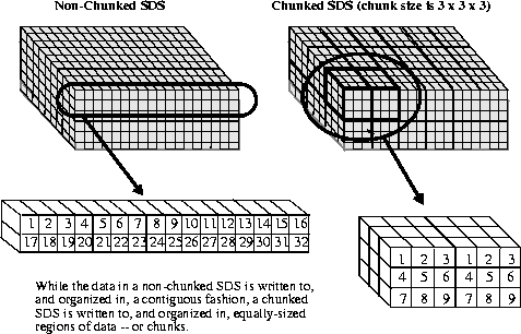
The following figure illustrates the difference between a non-chunked SDS and a chunked SDS.
FIGURE 14i - Comparison between Chunked and Non-chunked Scientific Data Sets

14.3.2 Writing Concerns and Reading Concerns in Chunking
There are issues in working with chunks that are related to the reading process and others that are related to the writing process.
Specifically, the issues that affect the process of reading from chunked SDSs are
The issues that affect the process of writing to chunked SDSs are
14.3.3 Chunking without Compression
Accessing Subsets According to Storage Order
The main consideration to keep in mind when subsetting from chunked and non-chunked SDSs is that if the subset can be accessed in the same order as it was stored, subsetting will be efficient. If not, subsetting may result in less-than-optimal performance considering the number of elements to be accessed.
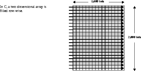
To illustrate this, the instance of subsetting in non-chunked SDSs will first be described. Consider the example of a non-chunked, two-dimensional, 2,000 x 1,600 SDS array of integer data. The following figure shows how this array is filled with data in a row-wise fashion. (Each square in the array shown represents 100 x 100 integers.)
FIGURE 14j - Filling a Two-dimensional Array with Data Using Row-major Ordering

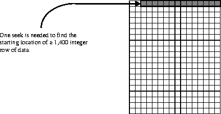
The most efficient way an application can read a row of data, or a portion of a row, from this array, is a contiguous, row-wise read of array elements. This is because this is the way the data was originally written to the array. Only one seek is needed to perform this. (See Figure 14k.)
FIGURE 14k - Number of Seeks Needed to Access a Row of Data in a Non-chunked SDS

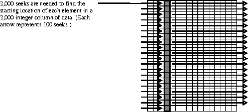
If the subset of data to be read from this array is one 2,000 integer column, then 2,000 seeks will be required to complete the operation. This is the most inefficient method of reading this subset as nearly all of the array locations will be accessed in the process of seeking to a relatively small number of target locations.
FIGURE 14l - Number of Seeks Needed to Access a Column of Data in a Non-chunked SDS

Now suppose this SDS is chunked, and the chunk size is 400 x 400 integers. A read of the aforementioned row is performed. In this case, four seeks are needed to read all of the chunks that contain the target locations. This is less efficient than the one seek needed in the non-chunked SDS.
FIGURE 14m - Number of Seeks Needed to Access a Row of Data in a Chunked SDS

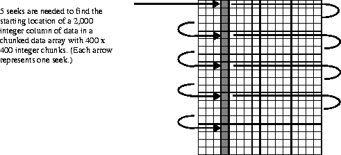
To read the aforementioned column of data, five chunks must be read into memory in order to access the 2,000 locations of the subset. Therefore, five seeks to the starting location of each of these chunks are necessary to complete the read operation, far fewer than the 2,000 needed in the non-chunked SDS.
FIGURE 14n - Number of Seeks Needed to Access a Column of Data in a Chunked SDS

These examples show that, in many cases, chunking can be used to reduce the I/O overhead of subsetting, but in certain cases, chunking can impair I/O performance.
The efficiency of subsetting from chunked SDSs is partly determined by the size of the chunk: the smaller the chunk size, the more seeks will be necessary. Chunking can substantially improve I/O performance when data is read along the slowest-varying dimension. It can substantially degrade performance when data is read along the fastest-varying dimension.
14.3.4 Chunking with Compression
Chunking can be particularly effective when used in conjunction with compression. It allows subsets to be read (or written) without having to uncompress (or compress) the entire array.
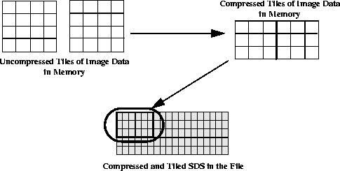
Consider the example of a tiled, two-dimensional SDS containing one million bytes of image data. Each tile of image data has been compressed as illustrated in the following figure.
FIGURE 14o - Compressing and Writing Chunks of Data to a Compressed and Tiled SDS

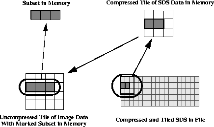
When it becomes necessary to read a subset of the image data, the application passes in the location of a tile, reads the entire tile into a buffer, and extracts the data-of-interest from that buffer.
FIGURE 14p - Extracting a Subset from a Compressed and Tiled SDS

In a compressed and non-tiled SDS, retrieving a subset of the compressed image data necessitates reading the entire contents of the SDS array into a memory buffer and uncompressing it in-core. (See Figure 14q.) The subset is then extracted from this buffer. (Keep in mind that, even though the illustrations show two-dimensional data tiles for clarity, this process can be extended to data chunks of any number of dimensions.)
FIGURE 14q - Extracting a Subset from a Compressed Non-tiled SDS

As compressed image files can be as large as hundreds of megabytes in size, and a gigabyte or more uncompressed, it is clear that the I/O requirements of reading to and writing from non-tiled, compressed SDSs can be immense, if not prohibitive. Add to this the additional I/O burden inherent in situations where portions of several image files must be read at the same time for comparison, and the benefits of tiling become even more apparent.
NOTE: It is recommended that the SDwritechunk routine be used to write to a compressed and chunked SDS. SDwritechunk can perform this operation more efficiently than the combination of SDsetcompress and SDwritedata. This is because the chunk information provided by the user to the SDwritechunk routine must be retrieved from the file by SDwritedata, and therefore involves more computational overhead.
14.3.5 Effect of Chunk Size on Performance
The main concern in modelling data for chunking is that the chunk size be approximately equal to the average expected size of the data block needed by the application.
If the chunk size is substantially larger than this, increased I/O overhead will be involved in reading the chunk and increased performance overhead will be involved in the decompression of the data if it is compressed. If the chunk size is substantially smaller than this, increased performance and memory/disk storage overhead will be involved in the HDF library's operations of accessing and keeping track of more chunks, as well as the danger of exceeding the maximum number of chunks per file. (64K)
It is recommended that the chunk size be at least 8K bytes.
14.3.6 Insufficient Chunk Cache Space Can Impair Chunking Performance
The HDF library provides caching chunks. This can substantially improve I/O performance when a particular chunk must be accessed more than once.
There is a potential performance problem when subsets are read from chunked datasets and insufficient chunk cache space has been allocated. The cause of this problem is the fact that two separate levels of the library are working to read the subset into memory and these two levels have a different perspective on how the data in the dataset is organized.
Specifically, higher-level routines like SDreaddata access the data in a strictly row-wise fashion, not according to the chunked layout. However, the lower-level code that directly performs the read operation accesses the data according to the chunked layout.
As an illustration of this, consider the 4 x 12 dataset depicted in the following figure.
FIGURE 14r - Example 4 x 12 Element Scientific Data Set

Suppose this dataset is untiled, and the subset shown in the following figure must be read.
FIGURE 14s - 2 x 8 Element Subset of the 4 x 12 Scientific Data Set

As this dataset is untiled, the numbers are stored in linear order. SDreaddata finds the longest contiguous stream of numbers, and requests the lower level of the library code to read it into memory. First, the first row of numbers will be read:
3 4 5 6 7 8 9 10
Then the second row:
23 24 25 26 27 28 29 30
This involves two reads, two disk accesses and sixteen numbers.
Now suppose that this dataset is tiled with 2 x 2 element tiles. On the disk, the data in this dataset is stored as twelve separate tiles, which for the purposes of this example will be labelled A through L.
FIGURE 14t - 4 x 12 Element Data Set with 2 x 2 Element Tiles

Also, the chunk cache size is set to 2.
A request is made to read the aforementioned subset of numbers into memory. As before, SDreaddata will determine the order the numbers will be read in. The routine has no information about the tiled layout. The higher-level code will again request the values in the first rows of tiles B through E from the lower level code on the first read operation.
In order to access those numbers the lower level code must read in four tiles: B, C, D, E. It reads in tiles B and C, retrieving the values 3, 4, 5, and 6. However, as the cache space is now completely filled, it must overwrite tile B in the cache to access the values 7 and 8, which are in tile D. It then has to overwrite tile C to access the values 9 and 10, which are in tile E. Note that, in each case, half of the values from the tiles that are read in are unused, even though those values will be needed later.
Next, the higher-level code requests the second row of the subset. The lower-level code must reread tile B to access the values 23 and 24. But tile B is no longer in the chunk cache. In order to access tile B, the lower-level code must overwrite tile D, and so on. By the time the subset read operation is complete, it has had to read in each of the tiles twice. Also, it has had to perform 8 disk accesses and has read 32 values.
Now consider a more practical example with the following parameters:
If the dataset is untiled the numbers are read into memory row-by-row. This involves 300 disk accesses for 300 rows, with each disk access reading in 1,000 numbers. The total number of numbers that will be read is 300,000.
Suppose the dataset is tiled as follows:
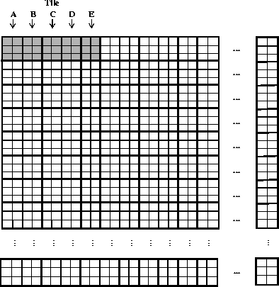
Each square in the following figure represents one 100 x 100 element region of the dataset. Five tiles span the 300 x 1,000 target subset. For the purposes of this example, they will be labelled A, B, C, D and E.
FIGURE 14u - 5 200 x 300 Element Tiles Labelled A, B, C, D and E

First, the higher-level code instructs the lower-level code to read in the first row of subset numbers. The lower-level code must read all five tiles (A through E) into memory, as they all contain numbers in the first row. Tiles A and B are read into the cache without problem, then the following set of cache overwrites occurs.
- Tile A is overwritten when tile C is read.
- Tile B is overwritten when tile D is read.
- Tile C is overwritten when tile E is read.
When the first row has been read, the cache contains tiles D and E.
The second row is then read. The higher-level code first requests tile A, however the cache is full, so it must overwrite tile D to read tile A. Then the following set of cache overwrites occur.
- Tile E is overwritten when tile B is read.
- Tile A is overwritten when tile C is read.
- Tile B is overwritten when tile D is read.
- Tile C is overwritten when tile E is read.
For each row, five tiles must be read in. No actual caching results from this overwriting. When the subset read operation is complete, 300 * 5 = 1,500 tiles have been read, or 60,000 * 1,500 = 90,000,000 numbers.
Essentially, five times more disk accesses are being performed and 900 times more data is being read than with the untiled 3,000 x 8,400 dataset. The severity of the performance degradation increases in a non-linear fashion as the size of the dataset increases.
From this example it should be apparent that, to prevent this kind of chunk cache "thrashing" from occurring, the size of the chunk cache should be made equal to, or greater than, the number of chunks along the fastest-varying dimension of the dataset. In this case, the chunk cache size should be set to 4.
When a chunked SDS is opened for reading or writing, the default cache size is set to the number of chunks along the fastest-varying dimension of the SDS. This will prevent cache thrashing from occurring in situations where the user does not set the size of the the chunk cache. Caution should be exercised by the user when altering this default chunk cache size.
[Top] [Prev] [Next]
hdfhelp@ncsa.uiuc.edu
HDF User's Guide - 05/19/99, NCSA HDF
Development Group.
